Nose Cone Shape Optimisation
This page illustrates how pysagas can be used for design optimisation. The example is applied to a nose cone at an operating point of Mach 6, 0 degrees angle-of-attack.
Literature Review
A review of literature reveals that the optimal shape for an axisymmetric nose at supersonic speeds which minimises drag for a given length and base diameter is given by the exponential function:
The exponent \(n\) depends weakly on the Mach number: for Mach 2-4, \(n\) should be approximately \(0.68\); for Mach >4, \(n \approx 0.69\)[1]. When \(n=1\), a sharp cone is produced.
The difference in drag for these exponnents is very slim, so previous experimental studies have made approximations with \(n=0.75\)[2],[3].

Geometry Definition
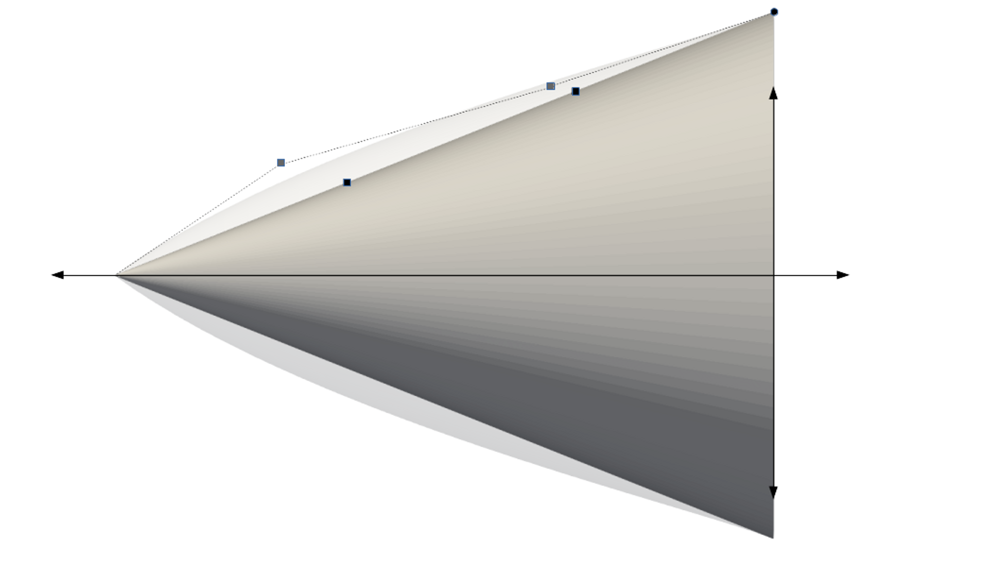
The nose geometry is defined by a Bezier curve with two internal control points, as shown in the figure below. These control points can move in both the horizontal and vertical direction. Therefore, there are 4 design parameters in this problem.
Optimisation Process
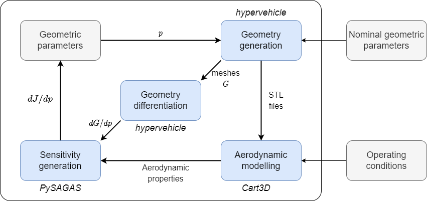
The optimisation process follows the schematic in the figure below.
Starting with a nominal set of geometric parameters,
HyperVehicle is used
to generate STL files. These files are passed into an aerodynamic modelling
package, in order to obtain the nominal flow solution for that geometry.
HyperVehicle is also
used to generate the geometry sensitivities, \(dv/dp\), which are used in
conjunction with the flow solution to generate the design parameter
sensitivities via pysagas. Finally, these sensitivities can be
passed into an optimisation algorithm to update the geometric parameters,
and perform another update iteration. The loop will continue until
some convergence tolerance is satisfied, at which point the optimal
geometry will have been reached. This loop has been implemented in
pysagas.optimisation.cartd.ShapeOpt.
In this example, the objective function is the drag coefficient of the nose cone, neglecting the base drag (as per the prior art).
Geometry Generation and Differentiation
As mentioned above, the geometry and geometry-parameter sensitivities, \(dv/dp\), will be generated using the parametric geometry generation package, HyperVehicle. This package allows a user to parametrically define a vehicle and output STL files for aerodynamic modelling.
Aerodynamic Modelling
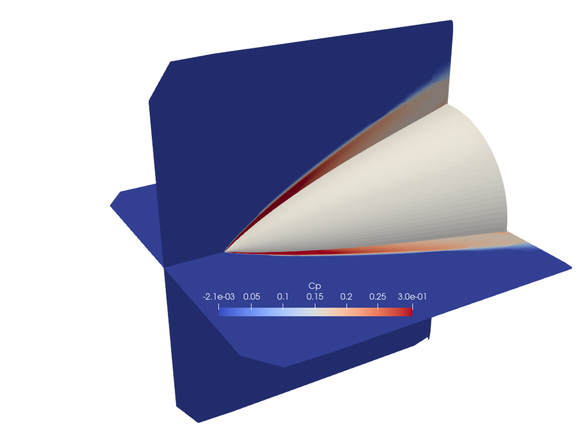
Given the STL files from the geometry generation module, the geometry will be simulated in the inviscid CFD solver, Cart3D. The figure below shows an example mesh produced by Cart3D.

The corresponding flow solution for this mesh is visualised in the figure below.
Results
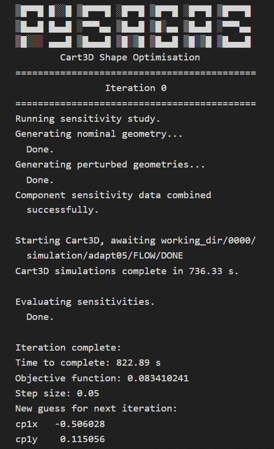
With the modules described above in place, the following output will
be displayed when running ShapeOpt.
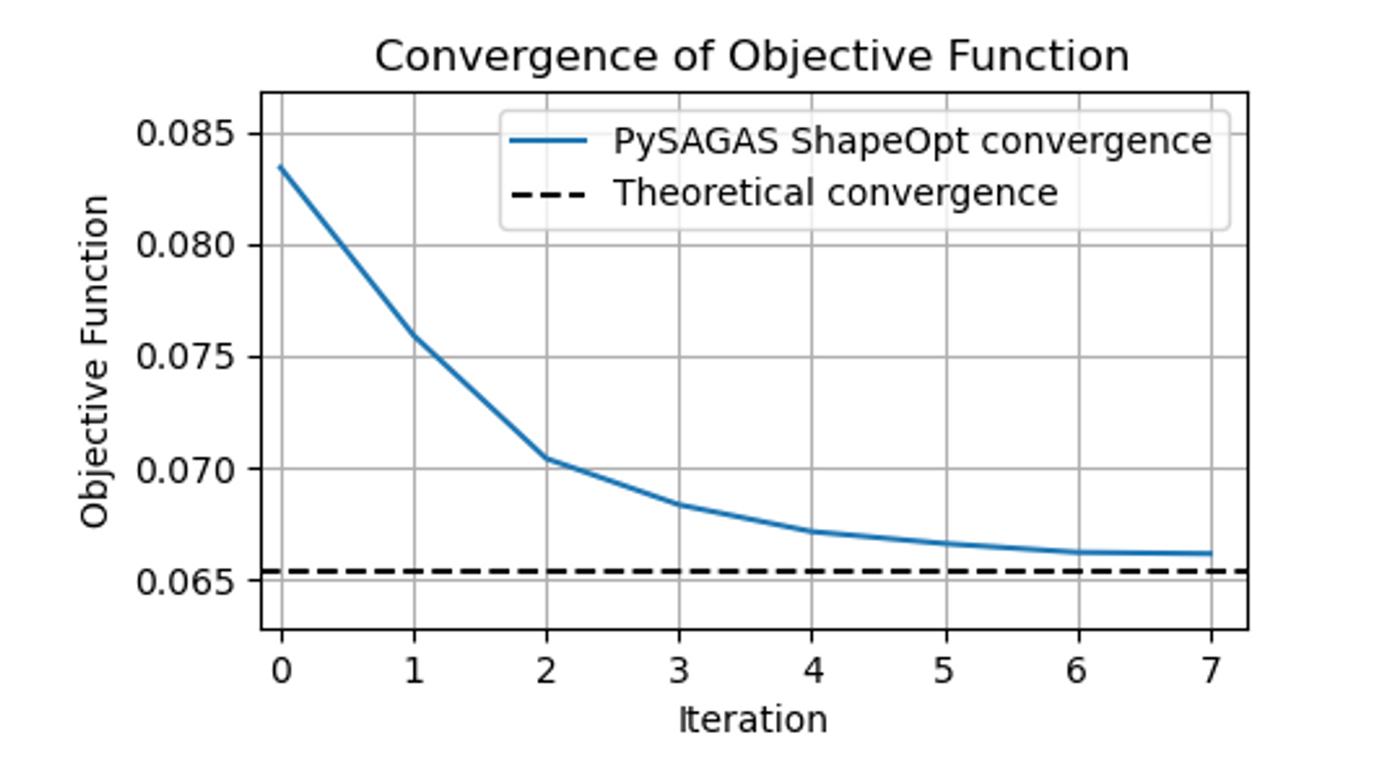
After 7 iterations, the following convergence plot can be created. Also shown on this plot is the ‘theoretical convergence’, which refers to the drag coefficient of the nose defined by the exponential function above, when simulated in the same manner used in the optimisation.
Finally, the nose geometry produced by pysagas can be compared to the theoretical optimal nose geometry, defined by the exponential function above. This comparison is shown in the figure below.
